Aerodrome charts with R and OSM

During my day-time job I deal with operational performance at airports. One recurring graphical requirement is to plot the aerodrome layout. It follows from this post that there is no ready-out-of-the-box solution for this task.

OpenStreetMap provides geographical information organised in layers. These layers can be querried for further processing.

The following code snippets shows the OSM query for extracting the feature aeroway and associated elements such as apron, gate, etc.
Consult the documentation to learn more about these element labels.

# setup
library(tidyverse)
library(osmdata)

# OSM query
bb_lonlat <- c(-0.223915,51.141733,-0.155851,51.165738)
apt_icao  <- "EGKK"
apt_name  <- "London Gatwick"

q <- opq(bbox = bb_lonlat) %>% 
  add_osm_feature(
    key = "aeroway"
    ,value =c("aerodrome", "apron", "control_tower", "gate", "hangar"
              ,"helipad", "runway", "taxiway", "terminal") ) %>% 
  osmdata_sf() %>%
  unique_osmdata()

1. identify the region of the world you are interested in. Here we use bboxfinder.com to zoom in on London Gatwick airport. With the draw rectangle we identify the bounding box to limit the query to the part of the world we are interested in! Please ensure that you select (or code) the lnglat format (longitude, latitude rather than the geographic convention latitude before longitude!).
2. we supply the bounding box coordinates bb_lnglat to the ‘opq()’ function which queries the OpenStreetMap database.
3. for the chosen bounding box we query for the respective feature(s) we are interested, i.e. ‘add_osm_feature(key = “my-key-of-interest”, value = “key-or-keys-of-interest”)’. Multiple feature keys can be grouped together by contaniation ‘c()’.
4. with ‘osmdata_sf()’ the extracted features will be coerced into sf objects.
5. ‘unique_osmdata()’ removes potential duplicate entries based on the use of multipoints/points, multistringlines/lines, etc that may result in double entries (spatial positions).

The query results is stored in a variable ‘q’.

In the next step we draw the sf_objects extracted with the osm query.

g <- ggplot() +
  geom_sf(data = q$osm_polygons
          ,inherit.aes = FALSE
          ,color = "lightblue"
          #,fill  = "lightblue"
          ) +
  geom_sf(data = q$osm_lines %>% filter(aeroway != "runway")
          , color = "grey"
          ) +
  geom_sf(data = q$osm_lines %>% filter(aeroway == "runway"),
          inherit.aes = FALSE,
          color = "black",
          size = 2 #.4
          ,alpha = .8) +
  theme_void() +
  labs(title = "EGKK")

g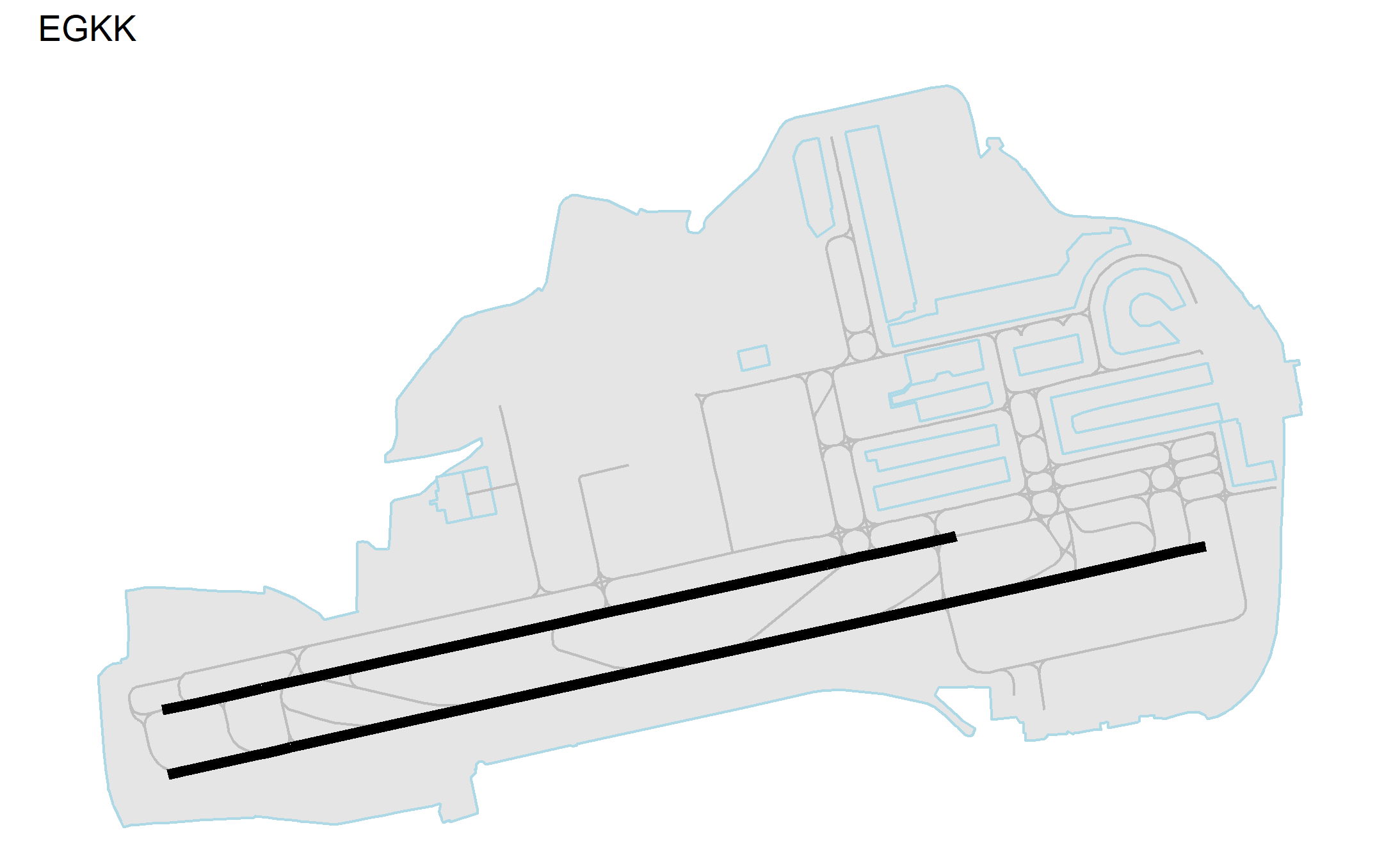

aerodrome chart of London Gatwick (EGKK)

If desired the generated aerodrome chart can be saved with the built-in ‘ggsave()’ function. For example:

fn <- paste(apt_icao, ".png", sep = "")
ggsave(filename = fn, path = "data-ad-charts")

As we have a ggplot the graph can be augmented with additional annotations. Furthermore the display, colouring, etc. of the different elements can be controlled via the ‘geom_sf()’ options. Have fun!